

Take a breath. If this chapter has been sitting in your syllabus looking like a wall of formulas — APC, MPS, multiplier, deflationary gap — I promise you it is far gentler than it looks. Everything here grows out of one very ordinary human habit: when people earn a little more, they spend some of it and save the rest. That single sentence is the seed. Every formula in this chapter is just that idea written in shorthand, and once you see the seed, the whole tree makes sense.
By the time we finish, you will be able to write a consumption or saving function from a word problem, find equilibrium income two different ways and get the same answer both times, calculate the multiplier in your head, and explain excess and deficient demand with the confidence of someone who actually understands them rather than someone reciting them. This unit carries 12 of the 40 marks in Part A — the single largest unit in Introductory Macroeconomics — so the hours you put in here pay you back more than anywhere else in the paper. Let us begin.
- Aggregate Demand and Its Components
- The Consumption Function: APC and MPC
- The Saving Function: APS and MPS
- How APC, APS, MPC and MPS Fit Together
- Investment, Ex-Ante and Ex-Post
- Equilibrium Output: The AD = AS Approach
- Equilibrium Output: The S = I Approach
- The Investment Multiplier and How It Works
- Full Employment and Involuntary Unemployment
- Excess Demand and Deficient Demand
- Correcting the Gaps: Fiscal and Monetary Measures
- Practice Worksheet
Your Game Plan for This Chapter
- Get the vocabulary straight first. Spend twenty minutes only on what C, S, I, Y, AD and AS stand for. Most confusion later is really vocabulary confusion in disguise.
- Master the four ratios. APC, MPC, APS and MPS. Learn them as a family of four, not as four strangers, because they are bound together by two tiny identities you will never forget once you see why they are true.
- Find equilibrium income both ways. Do every equilibrium sum twice — once by AD = AS and once by S = I. When both give the same number, you know you have it right, and you have also just proved the two methods are the same idea.
- Then, and only then, meet the multiplier. It is one formula, but it is the formula examiners love most. Practise it until 1 divided by (1 minus MPC) is automatic.
- Learn excess and deficient demand as a story, not a list. Too much demand causes inflation; too little causes unemployment. Every cause, effect and cure hangs off that one sentence.
- Finish with the worksheet at the bottom with your book closed. That last step is where the marks actually get made.
Study Notes
1. Aggregate Demand and Its Components
Imagine standing at the gate of a very large factory that produces everything the country makes — rice, phones, haircuts, bus rides, all of it. Now ask one question: how much of this output does the whole country actually want to buy this year? That total planned spending is aggregate demand (AD). It is not what people wish they could buy; it is what they plan to spend given their incomes and circumstances.
Aggregate demand has four buyers standing at that factory gate, and it helps enormously to picture them as four different customers with four different reasons for buying.
| Component | Symbol | Who is spending | Everyday example |
|---|---|---|---|
| Private final consumption expenditure | C | Households, on goods and services for their own use | A family buying groceries, school shoes, a cinema ticket |
| Investment expenditure | I | Firms, on capital goods and additions to stock | A bakery buying a new oven; a shop adding to its inventory |
| Government expenditure | G | The government, on goods and services | Building a district hospital; paying teachers’ salaries |
| Net exports | X − M | Foreigners buying our goods, minus what we buy from abroad | Exported textiles minus imported crude oil |
So the full statement is AD = C + I + G + (X − M). Your syllabus, however, does most of its analysis in a two-sector economy — only households and firms, no government and no foreign trade. That is not laziness; it is good teaching. Strip away the complications and the machinery becomes visible. In that simplified world, AD = C + I, and almost every numerical you will meet in the board exam uses exactly that form.
(a) A household buys a washing machine for home use. → This is a consumer durable bought for personal use, so it is consumption (C).
(b) A laundry business buys the same washing machine to wash customers’ clothes. → Same machine, different purpose. It is a capital good used to produce a service, so it is investment (I).
(c) The state government builds a new flyover. → Government expenditure (G).
(d) An Indian firm sells software worth Rs 60 crore to a client in Singapore. → Exports (X), which adds to net exports.
Why it works: notice that (a) and (b) are the same physical object. What decides the category is never the item — it is always the buyer and the purpose. Hold on to that and this classification stops being guesswork.
Step 1 — Net exports = X − M = 180 − 230 = −50 crore. (A negative figure is perfectly normal; it simply means this economy imported more than it exported.)
Step 2 — AD = C + I + G + (X − M) = 900 + 250 + 400 + (−50)
Step 3 — AD = 1550 − 50 = Rs 1500 crore.
Why it works: imports are goods produced abroad, so the money spent on them is demand for someone else’s output. We subtract them so that AD measures demand for domestic output only.
2. The Consumption Function: APC and MPC
Here is the seed of the whole chapter. Think about your own household. Even in a month with no income at all, some spending still has to happen — food, rent, electricity. That unavoidable minimum is called autonomous consumption, written as C̄ (“C-bar”), and it is paid for out of past savings or borrowing. Then, as income arrives, spending rises on top of that floor — but not rupee for rupee, because a sensible household saves part of every increase.
Put those two pieces together and you have the consumption function:
Now, two ratios describe this relationship, and students mix them up constantly. Let us make the difference physical.
Average propensity to consume (APC) answers: out of the whole income, what share is consumed? It looks at the total picture. APC = C / Y.
Marginal propensity to consume (MPC) answers: out of the extra income, what share is consumed? It looks only at the change. MPC = ΔC / ΔY.
An analogy that sticks: APC is your batting average for the whole season. MPC is your strike rate in the over you are batting right now. The season average includes every past ball; the current strike rate cares only about what just happened.
| Point of difference | APC | MPC |
|---|---|---|
| Question it answers | What fraction of total income is consumed? | What fraction of additional income is consumed? |
| Formula | C ÷ Y | ΔC ÷ ΔY |
| Can it exceed 1? | Yes — whenever consumption exceeds income (below the break-even level) | No — a household cannot consume more than 100% of the extra rupee it receives |
| Can it be zero? | No — consumption is never zero, so C/Y is always positive | Yes, in theory, if the entire increase in income is saved |
| Behaviour as income rises | Falls, because the fixed autonomous part is spread over a bigger income | Stays constant in a straight-line consumption function |
At Y = 400: C = 120 + 0.6(400) = 120 + 240 = Rs 360 crore. APC = C/Y = 360/400 = 0.9.
At Y = 600: C = 120 + 0.6(600) = 120 + 360 = Rs 480 crore. APC = 480/600 = 0.8.
MPC: ΔC = 480 − 360 = 120; ΔY = 600 − 400 = 200. MPC = 120/200 = 0.6.
Why it works: look what happened. APC fell from 0.9 to 0.8, but MPC stayed at 0.6. In fact MPC is simply the coefficient of Y sitting in the equation — you can read it off without any calculation at all. APC falls because the fixed Rs 120 crore of autonomous consumption becomes a smaller slice of a larger income.
Step 1 — ΔY = 36,000 − 24,000 = Rs 12,000.
Step 2 — ΔC = 30,000 − 21,000 = Rs 9,000.
Step 3 — MPC = ΔC/ΔY = 9,000/12,000 = 0.75.
Step 4 — MPS = 1 − MPC = 1 − 0.75 = 0.25.
Why it works: the extra Rs 12,000 had nowhere else to go — Rs 9,000 was consumed and the remaining Rs 3,000 must have been saved. Check: 3,000/12,000 = 0.25, exactly the MPS we found. The two fractions have to add to one because every extra rupee is either spent or kept.
Step 1 — C = 120 + 0.6(200) = 120 + 120 = Rs 240 crore.
Step 2 — APC = 240/200 = 1.2.
Step 3 — Interpretation: consumption (240) exceeds income (200) by Rs 40 crore. The economy is dissaving — drawing on past savings or borrowing to pay for the shortfall. Saving here is negative: S = Y − C = 200 − 240 = −Rs 40 crore.
Why it works: APC greater than 1 is not an error, it is a description of a poor or struggling economy living beyond its current income. This is exactly why APC can exceed one while MPC never can.
3. The Saving Function: APS and MPS
Saving is not a separate decision. It is the leftover. Whatever income you do not consume is, by definition, saved: S = Y − C. That is not a theory anyone had to discover — it is arithmetic.
And because saving is the leftover, the saving function falls straight out of the consumption function. Watch this, because it is the single most useful trick in the chapter. Start with S = Y − C, then substitute C = C̄ + bY:
S = Y − (C̄ + bY) = −C̄ + (1 − b)Y
The two ratios mirror the consumption ones exactly. APS = S / Y is the share of total income saved. MPS = ΔS / ΔY is the share of extra income saved.
One more idea worth ten marks over your school career: the break-even level of income. This is the income at which consumption exactly equals income, so saving is zero. Below it the economy dissaves; above it, it saves. At break-even, APC = 1 and APS = 0.
Step 1 — derive: S = Y − C = Y − (120 + 0.6Y) = −120 + 0.4Y. So S = −120 + 0.4Y, and MPS = 0.4.
Step 2 — at Y = 400: S = −120 + 0.4(400) = −120 + 160 = Rs 40 crore. APS = 40/400 = 0.1.
Step 3 — at Y = 600: S = −120 + 0.4(600) = −120 + 240 = Rs 120 crore. APS = 120/600 = 0.2.
Step 4 — cross-check: at Y = 400 we found C = 360 earlier, and 360 + 40 = 400 ✓. At Y = 600, C = 480 and 480 + 120 = 600 ✓.
Why it works: APS rose from 0.1 to 0.2 as income grew, which is the exact mirror of APC falling from 0.9 to 0.8. Richer economies save a larger share — the dissaving burden of that fixed Rs 120 crore shrinks in relative terms.
Method 1 — set S = 0: −120 + 0.4Y = 0, so 0.4Y = 120, giving Y = 300.
Method 2 — set C = Y: 120 + 0.6Y = Y, so 120 = 0.4Y, giving Y = 300. Same answer, as it must be.
Verification: at Y = 300, C = 120 + 0.6(300) = 120 + 180 = 300. So C = Y ✓, S = 0 ✓, APC = 300/300 = 1 ✓, APS = 0/300 = 0 ✓.
Why it works: notice the shortcut hiding here. Break-even income = C̄ ÷ MPS = 120 ÷ 0.4 = 300. That formula works every time, because the autonomous consumption has to be exactly cancelled out by saving from income, and each rupee of income contributes MPS to saving.
4. How APC, APS, MPC and MPS Fit Together
You now have four ratios, and they are bound together by two identities so simple you could prove them at the dinner table. Do not memorise them — understand them once and they are yours for life.
Start from the fact that every rupee of income is either consumed or saved: Y = C + S. Divide the whole thing by Y:
Y/Y = C/Y + S/Y, which gives 1 = APC + APS.
Now take the same fact but for a change in income: ΔY = ΔC + ΔS. Divide by ΔY:
ΔY/ΔY = ΔC/ΔY + ΔS/ΔY, which gives 1 = MPC + MPS.
| If income is… | Then C vs Y | Saving | APC | APS |
|---|---|---|---|---|
| Below break-even | C > Y (dissaving) | Negative | Greater than 1 | Negative |
| At break-even | C = Y | Zero | Exactly 1 | Exactly 0 |
| Above break-even | C < Y | Positive | Less than 1 | Positive |
Step 1 — APC = C/Y, so C = APC × Y = 0.85 × 500 = Rs 425 crore.
Step 2 — S = Y − C = 500 − 425 = Rs 75 crore.
Step 3 — APS = 1 − APC = 1 − 0.85 = 0.15. Check directly: S/Y = 75/500 = 0.15 ✓.
Step 4 — MPC = 1 − MPS = 1 − 0.3 = 0.7.
Why it works: notice that APC and MPC here are different numbers (0.85 and 0.7) and that is completely normal — they measure different things. The identities only link APC with APS, and MPC with MPS. Never subtract APC from MPC or you will produce nonsense.
5. Investment, Ex-Ante and Ex-Post
Investment in economics does not mean buying shares or gold. It means adding to the country’s stock of physical capital — machines, buildings, tools — plus any addition to inventories of unsold goods. When a firm buys a new lathe or a shopkeeper’s godown fills up with stock, that is investment.
In this chapter investment is treated as autonomous: a fixed amount that does not change when income changes. Written as I = Ī. That is a simplification, and a deliberate one — it lets us see clearly how consumption drives the system while investment acts as the push from outside.
Now for a distinction that trips up thousands of students every year, and it need not trip up you. The words are Latin but the idea is everyday.
Ex-ante means “before the event” — what people plan or intend to do. Ex-post means “after the event” — what actually happened, measured after the fact.
Here is the analogy. On Sunday evening you plan to study four hours on Monday: that is ex-ante. On Monday night you count up and find you studied two and a half: that is ex-post. Plans and outcomes are different things, and macroeconomics has to keep them apart.
| Ex-ante (planned) | Ex-post (realised) |
|---|---|
| Refers to what buyers and sellers intend to do | Refers to what they actually did |
| Measured before the period begins | Measured after the period ends |
| Ex-ante saving need not equal ex-ante investment | Ex-post saving is always equal to ex-post investment |
| Equality holds only at the equilibrium level of income | Equality holds at every level of income, by accounting |
| This is the concept used to determine equilibrium | This is the concept used to record what occurred |
Ex-ante investment is the amount of investment that firms plan or intend to undertake during a period, decided in advance on the basis of expected demand and expected profits. Ex-post investment is the investment that has actually taken place during the period, measured after it has ended.
The two differ whenever firms guess wrongly about demand. Suppose firms plan to invest Rs 200 crore and produce accordingly, but households buy Rs 50 crore less than expected. Those unsold goods do not vanish — they remain with the firms as stock, and an addition to stock is investment. So ex-post investment becomes 200 + 50 = Rs 250 crore, made up of Rs 200 crore planned and Rs 50 crore unintended inventory investment.
It is exactly this unintended component that forces ex-post saving and ex-post investment to be equal at every level of income: whatever output is not consumed must physically end up either as planned capital formation or as unsold stock, and both count as investment. The equality is therefore an accounting identity, not a condition of equilibrium.
Why it works: the phrase to hold on to is “unintended inventory investment”. It is the shock absorber that keeps the books balanced when plans go wrong, and naming it explicitly is what earns the fourth mark.
6. Equilibrium Output: The AD = AS Approach
Aggregate supply (AS) is the total value of goods and services all producers plan to supply, and since producing output is what generates income, aggregate supply is simply national income itself: AS = Y. That equality feels strange the first time; sit with it for a moment. Every rupee a firm earns from selling output becomes somebody’s income — wages, rent, interest or profit. Output and income are two names for the same flow.
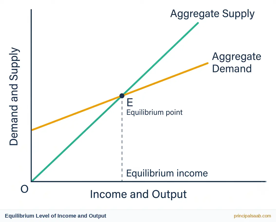
The economy is in equilibrium when what buyers plan to spend exactly matches what producers plan to supply: AD = AS, that is, C + I = Y.
Why does the economy settle there and nowhere else? Think about the two ways it can go wrong. If AD is greater than AS, buyers want more than firms produced; stocks run down below planned levels; firms notice and produce more; income rises. If AD is less than AS, goods pile up unsold; firms cut production; income falls. Only where AD = AS does nobody have a reason to change anything. The economy stops moving because it has run out of pressure.
At Y = 0: C = 100, AD = 100 + 100 = 200
At Y = 200: C = 200, AD = 200 + 100 = 300
At Y = 400: C = 300, AD = 300 + 100 = 400
At Y = 600: C = 400, AD = 400 + 100 = 500
At Y = 800: C = 500, AD = 500 + 100 = 600
Equilibrium is at Y = Rs 400 crore, the only row where AD equals Y (400 = 400).
Read the other rows as a story: below 400, AD exceeds output (at Y = 200, demand of 300 chases output of 200), so firms expand. Above 400, output exceeds AD (at Y = 800, output of 800 meets demand of only 600), so stocks build up and firms cut back. The economy is pushed towards 400 from both directions.
Why it works: AD rises by only 0.5 for every 1 rupee rise in Y, while AS rises by the full 1. Since AD starts above AS at low incomes and climbs more slowly, the two lines must cross exactly once — and that crossing is equilibrium.
Step 1 — write the equilibrium condition: Y = C + I
Step 2 — substitute: Y = 120 + 0.6Y + 80, so Y = 200 + 0.6Y
Step 3 — collect the Y terms: Y − 0.6Y = 200, so 0.4Y = 200
Step 4 — solve: Y = 200 ÷ 0.4 = Rs 500 crore
Step 5 — verify: at Y = 500, C = 120 + 0.6(500) = 120 + 300 = 420, so AD = 420 + 80 = 500 = Y ✓
Why it works: notice the shape of Step 4. Equilibrium income = (total autonomous spending) ÷ (1 − MPC) = (C̄ + Ī) ÷ MPS. Here that is 200 ÷ 0.4 = 500. Once you spot that pattern you can do these in one line — and you have also just met the multiplier without realising it.
7. Equilibrium Output: The S = I Approach
There is a second route to exactly the same destination, and understanding why it is the same route will do more for your confidence than any amount of memorising.
Start from the equilibrium condition Y = C + I. We also know, always and everywhere, that Y = C + S. If both are true at once, then C + S = C + I, and cancelling C from both sides leaves:
The intuition is worth a minute. Saving is a leakage — income that households receive but do not spend, so it drops out of the circular flow. Investment is an injection — spending that enters the flow from firms. If the leak is bigger than the top-up, the level of income falls. If the top-up is bigger than the leak, income rises. Income is stable only when the leak and the top-up are equal. Picture a water tank with a tap running in and a hole letting water out: the level holds steady only when inflow matches outflow.
Step 1 — derive the saving function: S = Y − C = Y − (120 + 0.6Y) = −120 + 0.4Y
Step 2 — apply S = I: −120 + 0.4Y = 80
Step 3 — solve: 0.4Y = 80 + 120 = 200, so Y = 200 ÷ 0.4 = Rs 500 crore
Step 4 — verify: S at Y = 500 is −120 + 0.4(500) = −120 + 200 = Rs 80 crore = I ✓
Why it works: the answer is Rs 500 crore, identical to Example 11 where we used AD = AS. This is not a coincidence and it is not luck — the two conditions are algebraically the same statement. Use this as your free self-check on every equilibrium numerical you ever attempt.
Step 1 — planned saving at Y = 700: S = −120 + 0.4(700) = −120 + 280 = Rs 160 crore.
Step 2 — compare: planned S (160) > planned I (80). The leakage exceeds the injection by Rs 80 crore.
Step 3 — check via AD: C = 120 + 0.6(700) = 540, so AD = 540 + 80 = Rs 620 crore, while output is Rs 700 crore. AD is short of AS by exactly Rs 80 crore.
Step 4 — what happens: Rs 80 crore of goods go unsold and accumulate as unintended inventory. Firms respond by cutting production, so income falls — and it keeps falling until it reaches Rs 500 crore, where planned S once again equals planned I.
Why it works: observe that the gap between planned S and planned I (80) is exactly the gap between AS and AD (80). That is the two approaches agreeing again, this time out of equilibrium. Note also that ex-post they are equal: realised investment is 80 planned + 80 unintended = Rs 160 crore, which matches realised saving of Rs 160 crore.
8. The Investment Multiplier and How It Works
Now the star of the chapter. Here is the question it answers: if investment in an economy rises by Rs 100 crore, by how much does national income rise? The instinctive answer is Rs 100 crore. The instinctive answer is wrong, and understanding why is the heart of this unit.
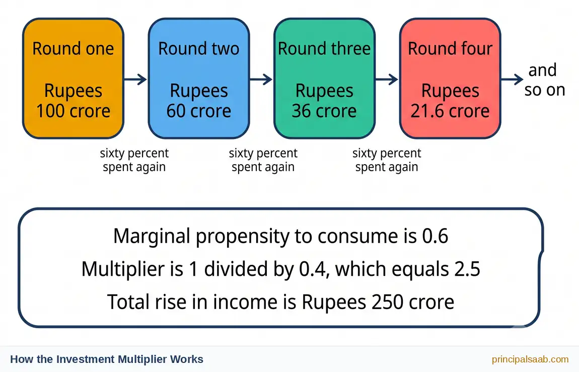
Follow the rupees. A firm spends Rs 100 crore building a factory. That money becomes income for builders, engineers and suppliers. Suppose the MPC is 0.6 — those people spend Rs 60 crore of it on food, clothes and rent. That Rs 60 crore becomes income for shopkeepers and landlords, who spend 60% of it, or Rs 36 crore. And so it rolls on, each round smaller than the last, but never quite reaching zero.
The investment multiplier (k) is the number that tells you the size of the total effect: k = ΔY / ΔI. And it can be calculated directly from the MPC:
Step 1 — k = 1/(1 − MPC) = 1/(1 − 0.6) = 1/0.4 = 2.5
Step 2 — ΔY = k × ΔI = 2.5 × 40 = Rs 100 crore
Step 3 — verify with the full model: using C = 120 + 0.6Y from before, investment rises from 80 to 120. New equilibrium: Y = 120 + 0.6Y + 120, so 0.4Y = 240, giving Y = Rs 600 crore. The old equilibrium was Rs 500 crore, so income rose by exactly Rs 100 crore ✓
Why it works: an injection of Rs 40 crore produced Rs 100 crore of extra income — two and a half times the original push. Nothing was created from nothing; the same rupees simply changed hands several times, and every time they changed hands they counted as somebody’s income.
Round 1: Rs 40.00 crore (the original investment)
Round 2: 0.6 × 40 = Rs 24.00 crore
Round 3: 0.6 × 24 = Rs 14.40 crore
Round 4: 0.6 × 14.4 = Rs 8.64 crore
Round 5: 0.6 × 8.64 = Rs 5.184 crore
Running total after five rounds: 40 + 24 + 14.4 + 8.64 + 5.184 = Rs 92.224 crore, and the rounds keep going, forever shrinking. The sum of the whole infinite series is 40 ÷ (1 − 0.6) = Rs 100 crore, exactly matching Example 14.
Why it works: each round is 60% of the one before, so this is a geometric series with first term 40 and common ratio 0.6. Its sum is a/(1 − r) = 40/0.4 = 100. The multiplier formula is nothing more mysterious than the sum of a geometric series — and the leakage into saving is what makes each round smaller and stops the process running away to infinity.
k = 1/MPS, so MPS = 1/k = 1/5 = 0.2, and MPC = 1 − 0.2 = 0.8.
(b) The MPS is 0.25 and the government wants national income to rise by Rs 800 crore. By how much must investment increase?
k = 1/0.25 = 4. Since ΔY = k × ΔI, we get ΔI = ΔY/k = 800/4 = Rs 200 crore.
Why it works: every multiplier question is one relationship, ΔY = k × ΔI, rearranged in one of three ways. Write that relationship down first, put in what you know, and the unknown falls out. There is genuinely nothing more to it.
9. Full Employment and Involuntary Unemployment
Everything so far has told us where the economy settles. Now comes the uncomfortable question that made this whole theory famous: is the place it settles a good place? Keynes’s answer, written while millions stood in dole queues during the Great Depression, was blunt: not necessarily.
Full employment does not mean every single person has a job. It means that everyone who is willing and able to work at the prevailing wage rate has found work. The income level at which this happens is called the full employment level of income, written YF. At full employment some unemployment still exists — people between jobs, or whose skills no longer match available work — but nobody is jobless simply because there is no work to be had.
Involuntary unemployment is the painful kind. It exists when people are willing to work at the going wage, are able to work, and actively want work — but cannot find a job, because aggregate demand is too low for firms to want to hire them.
| Voluntary unemployment | Involuntary unemployment |
|---|---|
| The person is not willing to work at the prevailing wage | The person is willing to work at the prevailing wage |
| Arises from personal choice or preference | Arises from insufficient aggregate demand in the economy |
| Not a policy problem — jobs are available | A serious policy problem — jobs are not available |
| Cannot be cured by raising demand | Can be cured by raising aggregate demand |
| Example: a graduate who declines offers to prepare for another exam | Example: a skilled weaver laid off because nobody is buying cloth |
Meaning: Involuntary unemployment is a situation in which workers who are willing and able to work at the existing wage rate are unable to find employment. The unemployment is not a matter of choice — the jobs simply do not exist.
How it persists in equilibrium: Equilibrium in this model means only that aggregate demand equals aggregate supply, so that firms have no reason to change their level of production. It carries no guarantee that this production level is high enough to employ the whole labour force.
Suppose the full employment level of income is Rs 2,000 crore, but aggregate demand is only sufficient to sustain an equilibrium income of Rs 1,600 crore. At Rs 1,600 crore firms are selling everything they produce, so they have no incentive to expand output, and therefore no incentive to hire more workers. The economy is stable, yet the labour needed to produce the missing Rs 400 crore of output stands idle. This is underemployment equilibrium.
Remedy: Because the cause is deficient aggregate demand, the cure must be to raise aggregate demand — for instance by increasing government expenditure or reducing taxes — so that equilibrium income rises towards YF.
Why it works: the answer earns full marks because it separates two ideas students routinely fuse: equilibrium (no tendency to change) and full employment (all willing workers employed). Making that separation explicit is the whole point of the question.
10. Excess Demand and Deficient Demand
We now have the two reference points we need: the equilibrium income the economy actually reaches, and the full employment income YF it ought to reach. Compare them and there are exactly three possibilities. One is comfortable; the other two are the problems this section is about.
Excess demand exists when aggregate demand exceeds the aggregate supply corresponding to full employment. The economy is already producing everything it possibly can, and still buyers want more. Output cannot rise — there are no idle workers or machines left — so the only thing that can rise is prices. The gap between AD and full-employment AS is called the inflationary gap.
Deficient demand exists when aggregate demand falls short of the aggregate supply corresponding to full employment. Buyers do not want everything the economy is capable of producing. Goods go unsold, firms cut production and lay off workers, and income falls below YF. The shortfall is called the deflationary gap.
A picture that may help: imagine a cinema hall with exactly 500 seats. If 600 people want tickets, you cannot create seats — ticket prices get bid up. That is excess demand. If only 380 people turn up, 120 seats sit empty and the staff hired for a full house have nothing to do. That is deficient demand.
| Basis | Excess demand | Deficient demand |
|---|---|---|
| Meaning | AD is greater than AS at the full employment level | AD is less than AS at the full employment level |
| Gap it creates | Inflationary gap | Deflationary gap |
| Effect on output | No change — output is already at its maximum | Output falls below the full employment level |
| Effect on employment | No change — already fully employed | Involuntary unemployment rises |
| Effect on prices | Prices rise, causing inflation | Prices tend to fall |
| Effect on inventories | Unplanned fall in inventories | Unplanned rise in inventories |
| Main causes | Rise in government spending, cut in taxes, rise in money supply, rise in exports | Fall in government spending, rise in taxes, fall in money supply, fall in exports |
| General remedy | Contractionary (tight) fiscal and monetary policy | Expansionary (easy) fiscal and monetary policy |
Method 1 — direct comparison at YF:
At Y = 2,500: C = 400 + 0.8(2,500) = 400 + 2,000 = Rs 2,400 crore
AD at YF = C + I = 2,400 + 200 = Rs 2,600 crore
AS at YF = Rs 2,500 crore
Inflationary gap = AD − AS = 2,600 − 2,500 = Rs 100 crore
Method 2 — via the multiplier:
Equilibrium income: Y = 400 + 0.8Y + 200, so 0.2Y = 600, giving Y = Rs 3,000 crore
k = 1/(1 − 0.8) = 1/0.2 = 5
Inflationary gap = (Y − YF) ÷ k = (3,000 − 2,500) ÷ 5 = Rs 100 crore ✓
Why it works: both methods give Rs 100 crore, and that agreement is the point. The gap is not the Rs 500 crore difference between equilibrium and full employment income — that is the eventual effect. The gap is the Rs 100 crore of excess demand which, multiplied by 5, produces that Rs 500 crore. Always divide by the multiplier, never forget to.
Method 1 — direct comparison at YF:
At Y = 1,200: C = 100 + 0.75(1,200) = 100 + 900 = Rs 1,000 crore
AD at YF = 1,000 + 150 = Rs 1,150 crore
AS at YF = Rs 1,200 crore
Deflationary gap = AD required at full employment − actual AD = 1,200 − 1,150 = Rs 50 crore
Method 2 — via the multiplier:
Equilibrium: Y = 100 + 0.75Y + 150, so 0.25Y = 250, giving Y = Rs 1,000 crore
k = 1/0.25 = 4
Deflationary gap = (YF − Y) ÷ k = (1,200 − 1,000) ÷ 4 = Rs 50 crore ✓
Interpretation: the economy comes to rest at Rs 1,000 crore while it is capable of Rs 1,200 crore. Output worth Rs 200 crore is never produced and the workers who would have produced it are involuntarily unemployed. A demand shortfall of just Rs 50 crore has cost the economy four times that in lost output.
Why it works: the multiplier cuts both ways. It magnifies increases in demand, and it magnifies decreases just as ruthlessly. That amplification is precisely why governments treat a small demand shortfall as worth acting on quickly.
11. Correcting the Gaps: Fiscal and Monetary Measures
If the disease is too much demand or too little demand, the cure is obvious in principle: push demand down, or pull it up. The interesting part is who does the pushing and with what. There are two sets of instruments, operated by two different authorities.
Fiscal policy is run by the government and works through its budget — how much it spends and how much it taxes. Monetary policy is run by the central bank (the Reserve Bank of India) and works through the supply and cost of money and credit.
Under each, the logic never changes. For excess demand you tighten: spend less, tax more, make credit scarce and dear. For deficient demand you loosen: spend more, tax less, make credit plentiful and cheap. Learn the direction once and every measure follows from it.
| Instrument | To correct excess demand (contractionary) | To correct deficient demand (expansionary) |
|---|---|---|
| Government spending | Decrease spending on public works and transfers, reducing AD directly | Increase spending on infrastructure and welfare, raising AD directly |
| Taxes | Raise taxes so disposable income and consumption fall | Cut taxes so disposable income and consumption rise |
| Public borrowing | Increase borrowing from the public to absorb purchasing power | Reduce borrowing, leaving more purchasing power with the public |
| Bank rate / repo rate | Raise it — borrowing becomes costlier, credit demand falls | Lower it — borrowing becomes cheaper, credit demand rises |
| Reverse repo rate | Raise it — banks park more funds with the central bank, leaving less money available for public credit | Lower it — banks are discouraged from parking funds with the central bank, freeing more money for public credit |
| Open market operations | Sell government securities, drawing money out of the system | Buy government securities, putting money into the system |
| CRR and SLR | Raise them, cutting banks’ lending capacity | Lower them, expanding banks’ lending capacity |
| Margin requirement | Raise it, so less can be borrowed against the same security | Lower it, so more can be borrowed against the same security |
Step 1 — find the multiplier: MPC = 0.75, so MPS = 0.25 and k = 1/0.25 = 4.
Step 2 — find the required rise in income: ΔY needed = 1,200 − 1,000 = Rs 200 crore.
Step 3 — find the required injection: ΔG = ΔY ÷ k = 200 ÷ 4 = Rs 50 crore.
Step 4 — verify: with G = 50 added, AD = 100 + 0.75Y + 150 + 50 = 300 + 0.75Y. Equilibrium: 0.25Y = 300, so Y = Rs 1,200 crore ✓ — exactly the full employment level.
Why it works: the required increase in spending equals the deflationary gap itself, Rs 50 crore. That is not a coincidence — the gap is the missing demand, and once you inject it the multiplier does the remaining work, turning Rs 50 crore into Rs 200 crore of income. This is the elegance of the theory, and examiners love to see the verification step in Step 4.
Meaning: Excess demand is a situation in which aggregate demand exceeds the aggregate supply corresponding to the full employment level of output. Since the economy is already using all its resources, output cannot rise further; the excess demand therefore raises the general price level. The gap between AD and full-employment AS is called the inflationary gap.
Fiscal measures
1. Reduction in government expenditure. The government cuts spending on public works, subsidies and transfer payments. Since government expenditure is a direct component of aggregate demand, cutting it lowers AD immediately, and the multiplier reduces income by a larger amount.
2. Increase in taxes. Raising direct taxes such as income tax reduces households’ disposable income. With less to spend, consumption expenditure falls, and aggregate demand falls with it.
Monetary measures
1. Increase in the repo rate (bank rate). When the central bank raises the rate at which it lends to commercial banks, banks raise their own lending rates. Borrowing becomes costlier, so households borrow less for consumption and firms borrow less for investment, reducing AD.
2. Open market sale of securities. The central bank sells government securities in the open market. Buyers pay for them out of their bank deposits, so cash flows out of the banking system, reducing banks’ capacity to create credit and therefore reducing aggregate demand.
Conclusion: All four measures act in the same direction — they reduce aggregate demand towards the full employment level of output, closing the inflationary gap and easing the pressure on prices.
Why it works: notice the structure — meaning first, then measures grouped under clear headings, each with a one-line mechanism explaining how it reduces AD, and a closing sentence tying them together. That mechanism sentence is where the marks live; simply naming the measures would earn barely half.
Practice Worksheet
Book closed, pen in hand. Attempt each question fully before you open the answer — the struggle is where the learning actually happens. If you get one wrong, do not just read the solution; close it and redo the question from scratch.
Show Answer
APC = C/Y = 360/400 = 0.9
MPC = coefficient of Y = 0.7
Saving: S = Y − C = 400 − 360 = Rs 40 crore. (Or derive the function: S = −80 + 0.3Y, so S = −80 + 120 = 40 ✓)
APS = S/Y = 40/400 = 0.1
MPS = 1 − MPC = 1 − 0.7 = 0.3
Check: APC + APS = 0.9 + 0.1 = 1 ✓ and MPC + MPS = 0.7 + 0.3 = 1 ✓
Show Answer
Step 2 — k = 1/MPS = 1/0.2 = 5
Step 3 — ΔY = k × ΔI = 5 × 250 = Rs 1,250 crore
National income rises by Rs 1,250 crore — five times the initial injection — because each round of spending passes 80% of the money on to the next round.
Show Answer
Step 2 — MPC = 1 − MPS = 1 − 0.25 = 0.75
Step 3 — If households become more thrifty, MPS rises and MPC falls. Since k = 1/MPS, a larger MPS gives a smaller multiplier. For instance, if MPS rose to 0.5, k would fall to 2.
More saving means more leakage from the circular flow at every round, so each round of spending is smaller and the total effect on income is weaker.
Show Answer
Y = C + I = 150 + 0.75Y + 250
Y − 0.75Y = 400, so 0.25Y = 400
Y = 400 ÷ 0.25 = Rs 1,600 crore
S = I approach:
S = Y − C = Y − (150 + 0.75Y) = −150 + 0.25Y
Set S = I: −150 + 0.25Y = 250
0.25Y = 400, so Y = Rs 1,600 crore ✓
Verification: at Y = 1,600, C = 150 + 0.75(1,600) = 150 + 1,200 = Rs 1,350 crore. AD = 1,350 + 250 = Rs 1,600 crore = Y ✓. And S = 1,600 − 1,350 = Rs 250 crore = I ✓
Both methods must agree, because S = I is simply Y = C + I with C cancelled from both sides.
Show Answer
Step 2 — 200 = Y − 0.6Y = 0.4Y
Step 3 — Y = 200 ÷ 0.4 = Rs 500 crore
Step 4 — At Y = 500: C = 200 + 0.6(500) = 200 + 300 = Rs 500 crore, so S = 500 − 500 = 0.
Therefore APC = 500/500 = 1 and APS = 0/500 = 0.
Shortcut worth remembering: break-even income = autonomous consumption ÷ MPS = 200 ÷ 0.4 = 500.
Show Answer
Step 1 — MPS = 1 − 0.8 = 0.2, so k = 1/0.2 = 5
Step 2 — Shortfall in income = 5,000 − 4,400 = Rs 600 crore
Step 3 — Deflationary gap = shortfall in income ÷ k = 600 ÷ 5 = Rs 120 crore
Interpretation: aggregate demand is short of the full employment requirement by Rs 120 crore. Because the multiplier is 5, this modest shortfall in demand costs the economy Rs 600 crore of output and leaves the workers who would have produced it involuntarily unemployed.
Careful: the gap is Rs 120 crore, not Rs 600 crore. Always divide by the multiplier.
Show Answer
Ex-post saving is the saving that has actually taken place during the period. It is a realised magnitude, measured after the period has ended.
Key difference in behaviour: Ex-post saving is always equal to ex-post investment, because any output that is neither consumed nor sold ends up as unintended inventory investment, which balances the accounts by definition. Ex-ante saving, however, need not equal ex-ante investment — households and firms are different groups making independent decisions for entirely different reasons.
Condition for equality: Ex-ante saving equals ex-post saving only at the equilibrium level of income. At that income planned saving equals planned investment, so there is no unintended change in inventories and the planned and realised figures coincide. At any other income level they differ, and the difference is exactly the unintended inventory change that drives the economy back towards equilibrium.
Show Answer
Two causes (any two):
1. Increase in government expenditure without a matching rise in output — for example a large public works programme — which raises AD directly.
2. Reduction in taxes, which raises households’ disposable income and hence their consumption expenditure.
(Also acceptable: an increase in the money supply making credit cheap and plentiful; a rise in exports; a fall in the propensity to save.)
Two effects:
1. Rise in the general price level (inflation). Since the economy is already at full employment, output cannot expand to meet the extra demand, so the pressure falls entirely on prices.
2. No increase in output or employment. All resources are already fully employed, so real output and the level of employment remain unchanged — the effect is purely nominal.
(Also acceptable: an unplanned fall in inventories as stocks are drawn down; a fall in the real value of money, hurting fixed-income earners.)
Show Answer
Step 2 — 0.2Y = 150 + 50 = 200
Step 3 — Y = 200 ÷ 0.2 = Rs 1,000 crore
Step 4 — multiplier: MPS = 0.2 (the coefficient of Y in the saving function), so k = 1/0.2 = 5
Verification by AD = AS:
Since S = −50 + 0.2Y, the consumption function is C = Y − S = Y − (−50 + 0.2Y) = 50 + 0.8Y
Y = C + I = 50 + 0.8Y + 150, so 0.2Y = 200, giving Y = Rs 1,000 crore ✓
Check: C = 50 + 0.8(1,000) = Rs 850 crore, AD = 850 + 150 = Rs 1,000 crore = Y ✓
Show Answer
Numerical illustration (MPC = 0.5, ΔI = Rs 100 crore):
Multiplier k = 1/(1 − 0.5) = 1/0.5 = 2
Round 1: Rs 100 crore (the investment itself)
Round 2: 0.5 × 100 = Rs 50 crore
Round 3: 0.5 × 50 = Rs 25 crore
Round 4: 0.5 × 25 = Rs 12.5 crore
Round 5: 0.5 × 12.5 = Rs 6.25 crore, and so on.
Total = 100 + 50 + 25 + 12.5 + 6.25 + … = 100 ÷ (1 − 0.5) = Rs 200 crore
Conclusion: national income rises by Rs 200 crore, twice the initial investment of Rs 100 crore, so ΔY/ΔI = 2 = k ✓
Relationship with MPC: the multiplier depends entirely on the MPC. A higher MPC means less leakage into saving at each round, so each round is larger and the multiplier is bigger. At MPC = 0.8 the multiplier would be 5; at MPC = 0.5 it is only 2.
And that is the whole chapter. Look back at where you started — a page of intimidating abbreviations — and notice what you can do now: derive a saving function in one line, find equilibrium income two different ways and make them agree, and explain to somebody else why a Rs 50 crore shortfall in demand can cost an economy Rs 200 crore of output. That is real understanding, and it did not come from talent. It came from sitting down and working through it.
If some of it still feels shaky, that is completely normal and it is not a verdict on you. Pick the one section that feels weakest, redo its worked examples on paper tomorrow morning, and leave the rest alone. Progress in economics is not made in dramatic all-nighters — it is made by getting one more correct question than yesterday, every day, until the paper arrives and the questions look familiar. You are closer than you think. Keep going.